58. Optimal Growth II: Accelerating the Code with JAX#
In addition to what is in Anaconda, this lecture needs extra packages.
!pip install quantecon jax
58.1. Overview#
Previously, we studied a stochastic optimal growth model with one representative agent.
We solved the model using dynamic programming.
In writing our code, we focused on clarity and flexibility.
These are important, but there’s often a trade-off between flexibility and speed.
The reason is that, when code is less flexible, we can exploit structure more easily.
(This is true about algorithms and mathematical problems more generally: more specific problems have more structure, which, with some thought, can be exploited for better results.)
So, in this lecture, we are going to accept less flexibility while gaining speed, using just-in-time (JIT) compilation in JAX to accelerate our code.
Let’s start with some imports:
import matplotlib.pyplot as plt
import numpy as np
import jax
import jax.numpy as jnp
import jax.random as jr
from typing import NamedTuple
import quantecon as qe
58.2. The model#
The model is the same as in our previous lecture on optimal growth.
We use log utility in the baseline case.
We continue to assume that
\(f(k) = k^{\alpha}\)
\(\phi\) is the distribution of \(\xi := \exp(\mu + s \zeta)\) where \(\zeta\) is standard normal
We will once again use value function iteration to solve the model.
The algorithm is unchanged, but the implementation uses JAX.
As before, we will be able to compare with the true solutions
def v_star(y, α, β, μ):
    """
    True value function
    """
    c1 = np.log(1 - α * β) / (1 - β)
    c2 = (μ + α * np.log(α * β)) / (1 - α)
    c3 = 1 / (1 - β)
    c4 = 1 / (1 - α * β)
    return c1 + c2 * (c3 - c4) + c4 * np.log(y)

def σ_star(y, α, β):
    """
    True optimal policy
    """
    return (1 - α * β) * y
58.3. Computation#
We store primitives in a NamedTuple built for JAX and create a factory function to generate instances.
class OptimalGrowthModel(NamedTuple):
    α: float            # production parameter
    β: float            # discount factor
    μ: float            # shock location parameter
    s: float            # shock scale parameter
    γ: float            # CRRA parameter (γ = 1 gives log)
    y_grid: jnp.ndarray # grid for output/income
    shocks: jnp.ndarray # Monte Carlo draws of ξ


def create_optgrowth_model(α=0.4,
                           β=0.96,
                           μ=0.0,
                           s=0.1,
                           γ=1.0,
                           grid_max=4.0,
                           grid_size=120,
                           shock_size=250,
                           seed=0):
    """Factory function to create an OptimalGrowthModel instance."""

    key = jr.PRNGKey(seed)
    y_grid = jnp.linspace(1e-5, grid_max, grid_size)
    z = jr.normal(key, (shock_size,))
    shocks = jnp.exp(μ + s * z)

    return OptimalGrowthModel(α=α, β=β, μ=μ, s=s, γ=γ,
                              y_grid=y_grid, shocks=shocks)
We now implement the CRRA utility function, the Bellman operator and the value function iteration loop using JAX.
We also implement a golden section search for scalar maximization needed to solve the Bellman equation.
def u(c, γ):
    return jnp.where(jnp.isclose(γ, 1.0),
                     jnp.log(c), (c**(1.0 - γ) - 1.0) / (1.0 - γ))

def state_action_value(c, y, v, model):
    """
    Right hand side of the Bellman equation.
    """
    α, β, γ, shocks = model.α, model.β, model.γ, model.shocks
    y_grid = model.y_grid

    # Compute capital
    k = y - c

    # Compute next period income for all shocks
    y_next = (k**α) * shocks

    # Interpolate to get continuation values
    continuation = jnp.interp(y_next, y_grid, v).mean()

    return u(c, γ) + β * continuation

def golden_max(f, a, b, args=(), tol=1e-5, max_iter=100):
    """
    Golden section search for maximum of f on [a, b].
    """
    golden_ratio = (jnp.sqrt(5.0) - 1.0) / 2.0

    # Initialize
    x1 = b - golden_ratio * (b - a)
    x2 = a + golden_ratio * (b - a)
    f1 = f(x1, *args)
    f2 = f(x2, *args)

    def body(state):
        a, b, x1, x2, f1, f2, i = state

        # Update interval based on function values
        use_right = f2 > f1

        a_new = jnp.where(use_right, x1, a)
        b_new = jnp.where(use_right, b, x2)
        x1_new = jnp.where(use_right, x2,
                b_new - golden_ratio * (b_new - a_new))
        x2_new = jnp.where(use_right,
                a_new + golden_ratio * (b_new - a_new), x1)
        f1_new = jnp.where(use_right, f2, f(x1_new, *args))
        f2_new = jnp.where(use_right, f(x2_new, *args), f1)

        return a_new, b_new, x1_new, x2_new, f1_new, f2_new, i + 1

    def cond(state):
        a, b, x1, x2, f1, f2, i = state
        return (jnp.abs(b - a) > tol) & (i < max_iter)

    a_f, b_f, x1_f, x2_f, f1_f, f2_f, _ = jax.lax.while_loop(
        cond, body, (a, b, x1, x2, f1, f2, 0)
    )

    # Return the best point
    x_max = jnp.where(f1_f > f2_f, x1_f, x2_f)
    f_max = jnp.maximum(f1_f, f2_f)

    return x_max, f_max

@jax.jit
def T(v, model):
    """
    Bellman operator returning greedy policy and updated value
    """
    y_grid = model.y_grid

    def maximize_at_state(y):
        # Maximize RHS of Bellman equation at state y
        c_star, v_max = golden_max(state_action_value,
                                    1e-10, y - 1e-10,
                                    args=(y, v, model))
        return c_star, v_max

    v_greedy, v_new = jax.vmap(maximize_at_state)(y_grid)
    return v_greedy, v_new


@jax.jit
def vfi(model, tol=1e-4, max_iter=1_000):
    """Iterate on the Bellman operator until convergence."""
    y_grid = model.y_grid
    v0 = u(y_grid, model.γ)

    def body(state):
        v, i, err = state
        _, v_new = T(v, model)
        err = jnp.max(jnp.abs(v_new - v))
        return v_new, i + 1, err

    def cond(state):
        _, i, err = state
        return (err > tol) & (i < max_iter)

    v_final, _, _ = jax.lax.while_loop(cond, body, (v0, 0, tol + 1.0))
    c_greedy, v_solution = T(v_final, model)
    return c_greedy, v_solution
Let us compute the approximate solution at the default parameters
og = create_optgrowth_model()

with qe.Timer(unit="milliseconds"):
    c_greedy, _ = vfi(og)
    c_greedy.block_until_ready()
2535.73 ms elapsed
Here is a plot of the resulting policy, compared with the true policy:
fig, ax = plt.subplots()

ax.plot(og.y_grid, c_greedy, lw=2, alpha=0.8,
        label='approximate policy function')

ax.plot(og.y_grid, (1 - og.α * og.β) * og.y_grid,
        'k--', lw=2, alpha=0.8, label='true policy function')

ax.legend()
plt.show()
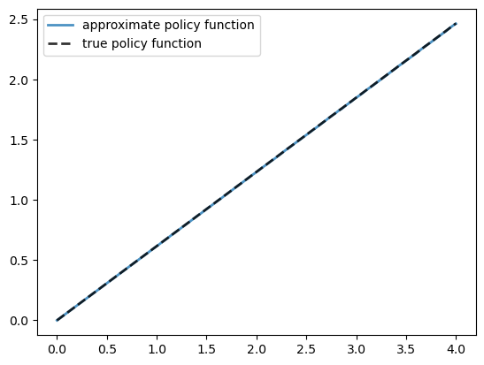
Again, the fit is excellent — this is as expected since we have not changed the algorithm.
The maximal absolute deviation between the two policies is
jnp.max(jnp.abs(c_greedy - (1 - og.α * og.β) * og.y_grid))
Array(0.00385427, dtype=float32)
58.4. Exercises#
Exercise 58.1
Time how long it takes to iterate with the Bellman operator 20 times, starting from initial condition \(v(y) = u(y)\).
Use the default parameterization and jax.lax.fori_loop for the iteration.
Solution to Exercise 58.1
Let’s set up the initial condition.
v = u(og.y_grid, og.γ)
Here is the timing.
with qe.Timer(unit="milliseconds"):
    def bellman_step(_, v_curr):
        return T(v_curr, og)[1]
    v = jax.lax.fori_loop(0, 20, bellman_step, v)
    v.block_until_ready()
675.05 ms elapsed
Compared with our timing for the non-compiled version of value function iteration, the JIT-compiled code is usually an order of magnitude faster.
Exercise 58.2
Modify the optimal growth model to use the CRRA utility specification.
Set γ = 1.5 as the default value while maintaining other specifications.
Use the JAX implementation above and change only the utility parameter.
Compute an estimate of the optimal policy and plot it.
Compare visually with the same plot from the analogous exercise in the first optimal growth lecture.
Compare execution time as well.
Solution to Exercise 58.2
Here is the CRRA variant using the same code path
og_crra = create_optgrowth_model(γ=1.5)
Let’s solve and time the model
with qe.Timer(unit="milliseconds"):
    c_greedy, _ = vfi(og_crra)
    c_greedy.block_until_ready()
1470.24 ms elapsed
Here is a plot of the resulting policy
fig, ax = plt.subplots()

ax.plot(og_crra.y_grid, c_greedy, lw=2, alpha=0.6,
        label='approximate policy function')

ax.legend(loc='lower right')
plt.show()
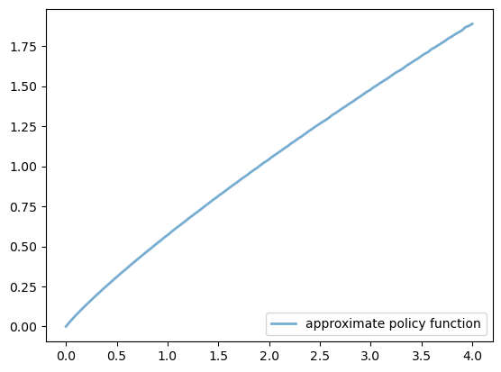
This matches the solution obtained in the non-jitted code in the earlier exercise.
Execution time is an order of magnitude faster.
Exercise 58.3
In this exercise we return to the original log utility specification.
Once an optimal consumption policy \(\sigma\) is given, income follows
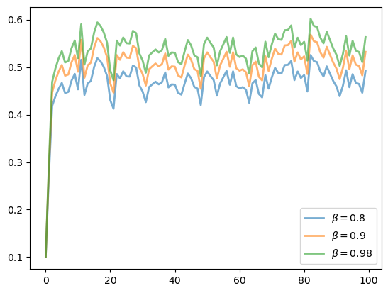
The next figure shows a simulation of 100 elements of this sequence for three different discount factors and hence three different policies.
In each sequence, the initial condition is \(y_0 = 0.1\).
The discount factors are discount_factors = (0.8, 0.9, 0.98).
We have also dialed down the shocks a bit with s = 0.05.
Other parameters match the log-linear model discussed earlier.
Notice that more patient agents typically have higher wealth.
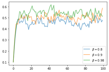
Replicate the figure modulo randomness.
Solution to Exercise 58.3
Here is one solution.
def simulate_og(σ_func, og_model, y0=0.1, ts_length=100, seed=0):
    """
    Compute a time series given consumption policy σ.
    """
    key = jr.PRNGKey(seed)
    ξ = jr.normal(key, (ts_length - 1,))
    y = np.empty(ts_length)
    y[0] = y0
    for t in range(ts_length - 1):
        y[t+1] = (y[t] - σ_func(y[t]))**og_model.α \
            * np.exp(og_model.μ + og_model.s * ξ[t])
    return y
fig, ax = plt.subplots()

for β in (0.8, 0.9, 0.98):

    og_temp = create_optgrowth_model(β=β, s=0.05)
    c_greedy_temp, _ = vfi(og_temp)

    σ_func = lambda x: np.interp(x, og_temp.y_grid,
                            np.asarray(c_greedy_temp))
    y = simulate_og(σ_func, og_temp)
    ax.plot(y, lw=2, alpha=0.6, label=rf'$\beta = {β}$')

ax.legend(loc='lower right')
plt.show()